


A method to assess epidemics and make decisions in epidemic prevention and control
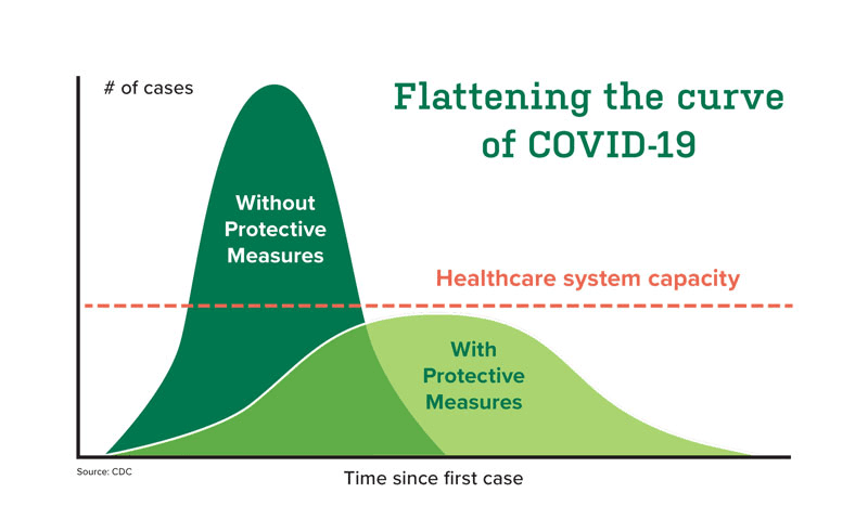
Table of contents
Article 1: A method to assess epidemics and make decisions in epidemic prevention and control
Article 2: An epidemic forecasting method
Article 3: Super-Spreading Waves
Website updating RT and other indicators operating since 21/09/2021 at onyx.vn/covid19/
A method to assess epidemics and make decisions in epidemic prevention and control
1. The basic reproduction number and the serial interval
For an epidemic, the basic reproduction number R0 and the average serial interval T are the two most important parameters. Let us start with an economics example. To assess economic growth, we compute GDP, and it is computed for a one-year period. For an epidemic, similarly we need to compute the two parameters R0 and T (the unit of T is days).
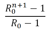
In the early stage of an epidemic, on average 1 infected individual produces R0 new infected individuals within T days. From that we can compute that, in the first n*T days, if R0 > 1, on average 1 infected individual produces a total of:

Example 1: COVID-19 variants have nearly the same average serial intervals, around 4, so we assume T = 4 [1,2]. For 20 days, we have n = 20 / T = 20 / 4 = 5.
The table below gives the total cases after 20 days for different values of R0 [3].
|
COVID-19 variant |
R0 |
Total cases after 20 days |
|
SARS-CoV-2 |
2 |
63 |
|
Alpha |
3.4 |
643 |
|
Delta |
5 |
3906 |
Example 2: A large R0 means little without T. The pair (R0 = 5, T = 4) makes cases rise faster than the pair (R0 = 25, T = 8), even though 25 is much larger than 5.
With large R0 and small T, cases rise very fast, so we must lock down more strictly when contact tracing capacity is exceeded.
2. Detecting an outbreak cluster
Suppose we cannot screen the whole population. How do we detect an outbreak cluster, and how many cases are in the cluster when we detect it?
To solve this problem, we need two more parameters besides R0 and T. Let p be the probability that a person will go to the hospital because of the disease. Let t be the average number of days from infection to hospital visit. For COVID-19, symptomatic cases make up at least 20% and severe cases at least 3%, so we tentatively assume p = 10%. For those who get COVID-19 with symptoms, symptoms appear on average 5 days after infection, so we assume t = 7.
First, let us compute the minimum number of cases needed to detect the cluster. Suppose we detect the cluster when an infected person goes to the hospital. The probability that a cluster of m people has no one going to the hospital is (1 - p)m (so we have not detected the cluster). Thus we need m = 29 for this probability to be 0.929 = 4.7% < 5%. That is, we detect the cluster with 95% probability when it has 29 cases.
Next, we convert the minimum case count into days. Assuming T = 4, the table below gives results for different values of R0.
|
COVID-19 variant |
R0 |
Days to reach at least 29 cases |
Days until hospital visit |
Total cases when the cluster is detected |
|
SARS-CoV-2 |
2 |
16 |
23 |
63 to 127 |
|
Alpha |
3.4 |
12 |
19 |
188 to 643 |
|
Delta |
5 |
8 |
15 |
156 to 781 |
With large R0, the case count when we detect the cluster is very large. In particular, cases rise very fast as seen in the previous section, so we must consider locking down quickly when tracing capacity is exceeded. The estimates will be more accurate if we estimate p and t instead of tentatively assuming them. This method does not require p to be very precise. For example, for the Delta variant, p from 10% to 20% gives the same results. However, if p = 5% (e.g., symptomatic but not going to hospital, or going to hospital but not necessarily detected) and t = 10, it would be a disaster for the Delta variant (total cases when the cluster is detected reach about 2600).
Finally, note that the total cases when the cluster is detected is only today's total, so future cases keep rising. Even if we apply lockdown measures and the reproduction number drops to 1, every 4 days, the total cases in the last 4 days (not the entire 781 cases in the Delta case) infect about as many more. The next section and the forecasting article will discuss this further.
3. Assessing the epidemic's progression through daily new cases
Above we assessed the risk when the epidemic just starts. This is feasible when a virus variant appears in our country after having appeared for a few months elsewhere. By then the parameters have already been estimated.
As the epidemic progresses, the number of immune people — from infection or vaccination — rises, and we also continuously change anti-epidemic measures. To assess the epidemic then, we do not use R0 but a more general coefficient: the effective reproduction number Re.
Let Vt be the new cases on day t. Assuming T = 4, Re at time t is estimated by the total cases of the next T days divided by the total cases of the latest T days (when the denominator is positive),

In the early stage of the epidemic, we have the following assessment table.
|
RT(t) |
Meaning |
|
RT(t) approximates R0 |
We are not intervening |
|
R0 > RT(t) > 1 but RT(t) shows no clear downward trend toward below 1 |
Our epidemic suppression is not good enough |
|
R0 > RT(t) > 1 and RT(t) clearly trends down toward below 1 over many days |
Epidemic suppression is progressing well |
|
1 > RT(t) |
We will have successfully suppressed the epidemic if we keep it up until no cases remain |
Similar to GDP in economics, RT can be computed for each region, province, or city, and it is affected by many factors such as masks, hygiene, population density, average travel distance, quarantine, distancing, etc. Therefore, we need further analyses to understand which factors affect the change in RT.
4. Applying to the outbreak since late April 2021
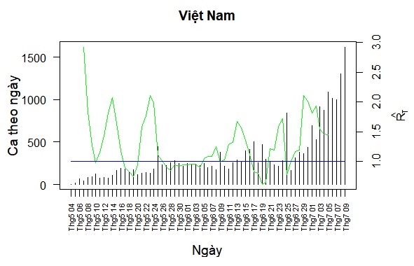
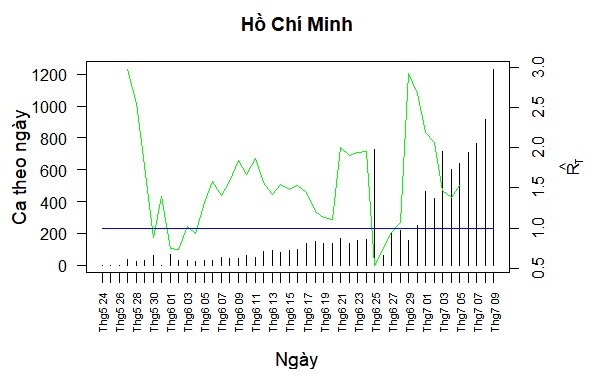
We compute RT for the COVID-19 outbreak in Vietnam (VN) that began in late April 2021. Daily new case data for Vietnam and each province/city are from VnExpress [4]. We discard about the first 4 to 7 values of RT because the data are unstable in the first days after a cluster is detected. We currently compute RT only for Vietnam and the two provinces/cities with the most cases, Bac Giang (BG) and Ho Chi Minh (HCM). When computing RT for a province, we ignore the error created by cases moving between provinces.
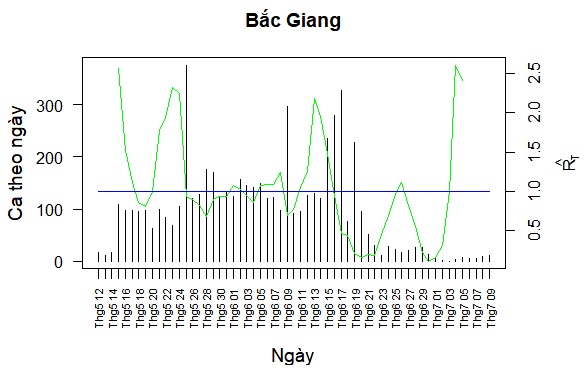
We observe three peaks of RT,VN on 14/5, 22/5, and 13/6, corresponding to three peaks of RT,BG. Two peaks of RT,VN on 24/6 and 29/6 correspond to two peaks of RT,HCM. This is why we need to analyze BG and HCM separately.
For BG, because initial testing capacity did not match quarantine capacity, RT,BG fluctuated strongly. However, RT,BG > 1 occurred only in periods of about a week, and notably there was a long period hovering around 1. This shows BG controlled the epidemic well.
For HCM, RT,HCM hovered around 1.5, so cases rose gradually. RT,HCM fell for about 4 days from 17/6 to 20/6 (but still above 1); however, this period is too short to be a trend. After more clusters were detected, RT,HCM immediately rose again. RT,HCM then fell below 1 for 4 days, but this was because detected cases were accumulated, not because of good epidemic control (a 4-day period is too short to show a trend). The biggest difference between BG and HCM is that HCM had no long period where RT,HCM truly hovered around 1 or clearly trended downward, which would show effective epidemic control.
For the Delta variant, as analyzed above, when a new cluster is detected through a patient going to hospital rather than screening, the case count in the cluster can be relatively large. Therefore, if we do not control RT well, we should plan new lockdown measures that are stronger and faster (compared with suppressing earlier COVID-19 variants).
5. Pooled testing
To reduce testing costs, we pool many samples together. The algorithm is: we test a pool of g samples; if negative, all samples in it are negative; if positive, we test each sample in it individually. Research shows we can pool up to 64 samples [5]. The question is: what is the optimal value of g?
We have not had time to give a satisfactory answer, so we only have a few tentative opinions. Let the total population be N and the proportion of cases in the population be q. For example, with N = 200 and only 1 case among them (q = 1/200), we have the following table.
|
g |
Number of tests needed |
|
1 |
200 |
|
10 |
20 + 10 = 30 |
|
15 |
19 to 29 |
|
20 |
10 + 20 = 30 |
|
40 |
5 + 40 = 45 |
|
200 |
1 + 200 = 201 |
We see that pooling more is not always better. The optimal value of g depends on q. The smaller q is, the larger the optimal g (the lower the case rate, the more samples we can pool).
The next observation is that the worst case occurs when each pool has only one case, because then the number of samples to test individually is the largest. When considering the worst case, we can reduce the above problem to a simpler problem as in the example above. Then the total population is 1/q with only 1 case.
To solve the general problem, we think simulation can be used.
6. Conclusion
Above we have presented in detail how to assess the risk when an epidemic starts and how to assess its progression. For more details, you can see the two attached slides. You can read how to estimate T and R0 in the references below. We apply these methods to the latest COVID-19 outbreak in Vietnam. We also briefly presented the optimal pooled sample size in testing. We will discuss other topics such as forecasting, testing methods, false positive/negative probabilities, vaccines, etc., in later articles.
- trunght@onyx.vn -
References
(See 11 more references in the 2 attached slides)
SIR (discrete time and changing parameters): SIR review - 210709.pdf
Assessing the epidemic's progression through daily new cases: time-since-infection model - 210710.pdf
1. Geismar, C. et al. Serial interval of COVID-19 and the effect of Variant B.1.1.7: analyses from a prospective community cohort study (Virus Watch). medRxiv 2021.05.17.21257223 (2021). doi:10.1101/2021.05.17.21257223
2. Pung, R., Mak, T. M., group, C. C.-19 working, Kucharski, A. J. & Lee, V. J. Serial intervals observed in SARS-CoV-2 B.1.617.2 variant cases. medRxiv 2021.06.04.21258205 (2021). doi:10.1101/2021.06.04.21258205
3. Wikipedia. Variants of SARS-CoV-2. Available at: https://en.wikipedia.org/wiki/Variants_of_SARS-CoV-2.
4. COVID-19 data in Vietnam. Available at: https://vnexpress.net/covid-19/covid-19-viet-nam. (Accessed: 10th July 2021)
5. Yelin, I. et al. Evaluation of COVID-19 RT-qPCR test in multi-sample pools. medRxiv 2020.03.26.20039438 (2020). doi:10.1101/2020.03.26.20039438