Super-Spreading Waves

In this article, we qualitatively and quantitatively evaluate a super-spreading event (SSE) through a real example.

SUPER-SPREADING WAVES

Many modelers and epidemiology researchers say that without super-spreading individuals/events (SSE) (superspreader/superspreading event), an epidemic would hardly break out.

In this article, we qualitatively and quantitatively evaluate a super-spreading event (SSE) through a real example. The SSE in Ho Chi Minh City (HCMC) on 07/08/2021 has created more than 10,000 infections to date, even without accounting for a time delay of about 10 days (and it will continue to create more infections until this outbreak ends).

We believe the SSE has both scientific and practical significance. The most important insight is a deeper understanding of the mechanism of epidemic spread, from which we can apply it in many ways for specific purposes. Scientifically, it helps us observe the serial interval, the wave cycle, the wave-like spread mechanism of epidemics, wave interference phenomena, and the social impacts that strengthen or weaken the waves. Practically, we hope the article helps everyone raise awareness of its harms and worry less when case numbers suddenly spike, as well as helping policymakers make better plans such as limiting gatherings before lockdown and choosing lockdown timing.

We have not had enough time to study this issue thoroughly; however, we decided to write this article early because of its practical significance. Some assumptions still need verification, so please read the guidance carefully before use.

1. Data

Our input data are the number of cases announced each day, the days lockdowns were imposed or lifted, the days of mass gathering events, and Google mobility ^1,2. The subject of study is the infection wave. A wave here is understood as the cyclic rise and fall of daily announced case numbers. An epidemic is the interaction between humans and the virus, so the wave depends on the virus's spread mechanism such as generation time (estimated by serial interval), as well as social behavior such as the 7-day cycle seen in many places around the world. The wave may also depend on data entry. You can view the Google chart, download the data for analysis, or see studies of this 7-day phenomenon ^3,4. Figure 1 shows case numbers over 30 days for the world, the US, and Vietnam. Case numbers are low on Wednesdays globally (on average). For the US (and Delhi, India / France), case numbers are low on weekends (and Mondays / Wednesdays, respectively). Thus this 7-day cycle depends on each society's behavior. It may be meeting more or less on certain days, the number of tests performed each day, or data entry (for example, fewer entries on weekends than weekdays).

Figure 1. Case numbers over 30 days for the world, the US, and Vietnam.

Thus two difficulties arise here. First, many waves interfere with each other, not counting noise or randomness. Second, each individual has 4 dates: the date of infection, the date of symptom onset, the date of detection, and the date of announcement (recording). The later dates are less accurate and cause distortion in the observed frequency of the wave.

To solve the first difficulty, we need to remove the 7-day cycle so the SSE wave shows more clearly (below we present a simulated example of the 7-day behavior cycle overpowering the 4-day SSE cycle). In Figure 1, Vietnam's data from JHU shows a 7-day wave with low case numbers on Mondays. However, data from the Ministry of Health for both Vietnam and HCMC do not show this (so the JHU data has some distortion). Moreover, among SSEs, one that occurs on a single day is the easiest to study. As mentioned in our previous article, we assume an SSE occurred on 07/08 in HCMC (all dates are in 2021). This SSE happened right before the lockdown. Imagine that the reproduction number would suddenly spike on the SS day and then fall to a lower level than before due to the lockdown. A wave with a dip right after a bump is even easier to observe. Thus HCMC data have many advantages for studying the SSE.

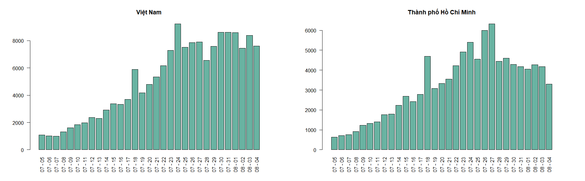
Figure 2. Daily case numbers over 30 days in Vietnam and HCMC

To solve the second problem, we assume that time intervals such as generation time, serial interval, and the recording interval are independent. Moreover, these intervals share the same distribution across cases. Thus announced cases still correctly reflect the epidemic's progression, but with a time delay. To deal with the problem of many unobserved infections, we assume the ratio between observations and actual figures does not change. Then R_T is unaffected because it is a ratio. These assumptions sound strict, but the model we use has matched reality across multiple outbreaks in Vietnam. It must also be said that the detection and recording dates for HCMC may not follow the same distribution across cases.

Finally, the dates lockdowns were imposed or lifted (we usually Google to find these past dates), the dates of major events, and Google mobility are used to find the days when social behaviors affected the epidemic's spread.

2. Methods and results

The main method is the model presented in Article 1, to which we add several assumptions. We assume an SSE occurred on 08/07 in HCMC as presented in the article of 18/07. We assume a delay of about 10 days between the infection date 08/07 and the announcement date 18/07. The reason is about 4 – 5 days of incubation, 2 days for pooled testing (day 1 pooled sample positive, day 2 individual samples), 2 – 3 days for contact tracing, and no more than 1 day for recording. Furthermore, we assume that without the super-spreading event, the case count on 18/07 would be at most 3,074 (we chose the case count of 19/07 as an upper bound because this number is neither too low nor too high, and is consistent with the observed upward average trend of case numbers). Thus at least 1,618 cases on 18/07 were contributed by the SSE. We assume all these cases can continue transmitting in future days. Note that more SSE cases may have been detected before 18/07 than after, so the number of cases caused by the SS may be higher than our estimates below.

2.1. Risk of infection in the SSE

Let V_t be the number of cases announced on a day. With a serial interval of 4, we roughly estimate the instantaneous reproduction number (see the slides attached to Article 1) to lie between:

4 * V_t/ (V_t-1 + V_t-2 + V_t-3 + V_t-4) and V_t/ V_t-4.

The reason is that most people infected today were infected by people who became infected within the previous 4 days.

We then compute the instantaneous reproduction number on 07/08 from the cases on 14-18/07. The result lies in the range (1.85 – 2.10). Without the super-spreading event, the case count on 18/07 would be 3,074, and the above range drops to (1.21 – 1.38). Thus the risk of being infected on the SS day 08/07 increased by about 50%. This number may not worry you much, but it is only today's number. It will feed into other numbers until this outbreak ends. Intuitively, people infected today will continue infecting others in the future, and the number of infected people will increase considerably. Then the probability of encountering a sick person also increases significantly if calculated over the whole outbreak period.

2.2. Cases added by the SSE

We present several methods to estimate the number of cases added by the SS.

Method 1 (upper bound): Future cases are mostly caused by the cases of the past 4 days. The total cases in the 4 days 15 – 18/07 is 12,589. Thus cases caused by the SS account for 1,618/12,589 = 12.9%. If we approximate that "future added cases are proportional to the cases added in the previous 4 days", then the SS contributed 12.9% of future cases. From 19/07 – 05/08, HCMC added 78,525 cases, so the SS created an additional 11,747 cases from 18/07 – 05/08. It will keep creating more cases until the outbreak ends. When simulating with the SEIR model, we see that future added cases account for a smaller share than the cases added in the previous 4 days. Therefore this number is an upper bound.

Method 2 (upper bound): Using data through 05/08, we estimate R_T up to 01/08. Every 4 days:

(cases on day t + 4) = (cases on day t) * (R_T on day t).

We then continue applying the same formula for days t + 8, t + 12, … Thus we compute a total of 11,962 cases through 03/08. For HCMC, R_T decreases over time, so this number is an upper bound.

Method 3 (lower bound): Identical to method 2 but we choose the smallest value of R_T:

(cases on day t + 4) = (cases on day t) * (R_T on day t + 3).

The reason is that R_T decreases over time for HCMC and R_T(t+3) is the last R_T related to day t. We compute a total of 9,599 cases through 03/08.

Method 4 (approximation): We estimate the smoothed red curve of R_T up to today. We then spread the cases evenly over the 4 days 11 – 14/07 and 15 – 18/07, and simulate with or without the 1,618 cases along the smoothed red curve of R_T (see the rationale for this method below). The result is 10,378 through 06/08.

Combining the above methods, we conclude that the SSE on 08/07 created more than 10,000 cases through 06/08 in HCMC (not yet adjusting for the 9 – 10 day delay between infection date and detection date). It will continue creating more cases until this outbreak ends.

2.3. Some assumptions through examples and real observations

We consider two simple examples (toy examples) to examine the properties of the SSE and social behavior.

Example 1: Suppose a person infected at time t only infects one other person at time t + 4. The case reproduction number (see the slides in Article 1) R_c starts at 1 for some days and decreases linearly by 0.02/day. Cases start at 100 cases/day. The SSE occurs on day 6 with 30 added cases.

Example 2: Suppose a person infected at time t only infects one other person at time t + 4. The case reproduction number R_c starts at 2 for some days then decreases linearly by 0.04/day. Cases start at 100 cases/day. Social behavior regarding meeting frequency varies within the week, making the reproduction number vary by 80%, 90%, 100%, 80%, 60%, 50%, 50% from Monday to Sunday.

We compute R_T without the SS (red curve), with the SS (green curve), and with a wrong R_T using cycles of 3 (blue curve) and 5 (purple curve). The results are in Figure 3.

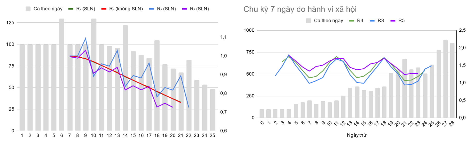
Figure 3. Results of example 1 on the left, example 2 on the right.

We have the following observations:

The SS makes daily case numbers show a positive wave. Wave peaks are 4 days apart.
The SS problem is equivalent to the intrusion problem (see the slides in Article 1). This is also shown by the green and red curves coinciding. This is why we applied the 4th method above.
If the wrong interval (3 or 5 instead of 4 days) is used to compute R_T, the R_T trajectory undulates. The wave cycle is always 4 days regardless of whether the interval used is 3 or 5 days. Computing R_T with 3 (5) days overestimates (underestimates) the true R_T when R_T,true < 1. This reverses when R_T,true > 1. This over/underestimation property still holds when we analyze this COVID wave's data in Vietnam. The serial interval is an important parameter. Previously we used serial intervals from other scientific reports. This method is another way to determine the serial interval.
Example 2 shows that the 7-day social behavior cycle can overpower the 4-day serial-interval cycle when observing the R_T trajectory.

2.4. Wave forecasting and case ups and downs caused by waves

First we recall a simple example of case ups and downs in the slides attached to Article 1.

Example 3: This example illustrates that today's case ups and downs relate to the cases 4 days ago, not yesterday's cases. In Figure 4, on day 5 (the first blue column), cases doubled compared to 4 days earlier, so the situation worsened. However, cases fell sharply compared to day 4 (the last green column). Conversely, on days 6 – 8, cases rose steadily, but the situation was improving. The reason is that cases halved compared to 4 days earlier.

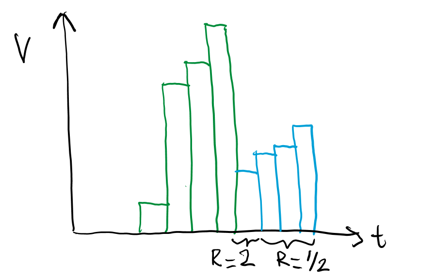
Figure 4. Cases fall compared to yesterday but the situation worsens, and vice versa

In this article, we forecast case ups and downs using HCMC data. Our method is simple: when there is a sudden spike in daily cases, we assume an SSE occurred. Based on the slopes of the smoothed red curve and the green curve for R_T, we estimate the future trend from the red curve and the wave cycle from the green curve. The wave height varies proportionally with the change of the red curve. The results are in Figure 5. Daily case numbers appear to rise in cycles of about 4 days for 3 consecutive rounds from 18 – 26/07, as described in example 2.

In Figure 5 on the left, on 03/08, we miscalculated the cycle because we had not accounted for Directive 16+ being applied on 24/07, which shifted the green curve's cycle. This led the estimated R_T curve to cross above 1 and create a second local peak. In Figure 5 on the right, on 05/08, after accounting for the impact of Directive 16+ and correcting the wave cycle, we predict cases will rise because R_T increases, but R_T will not exceed 1. The wave shape remains the same, but the wave peaks are considerably lower.

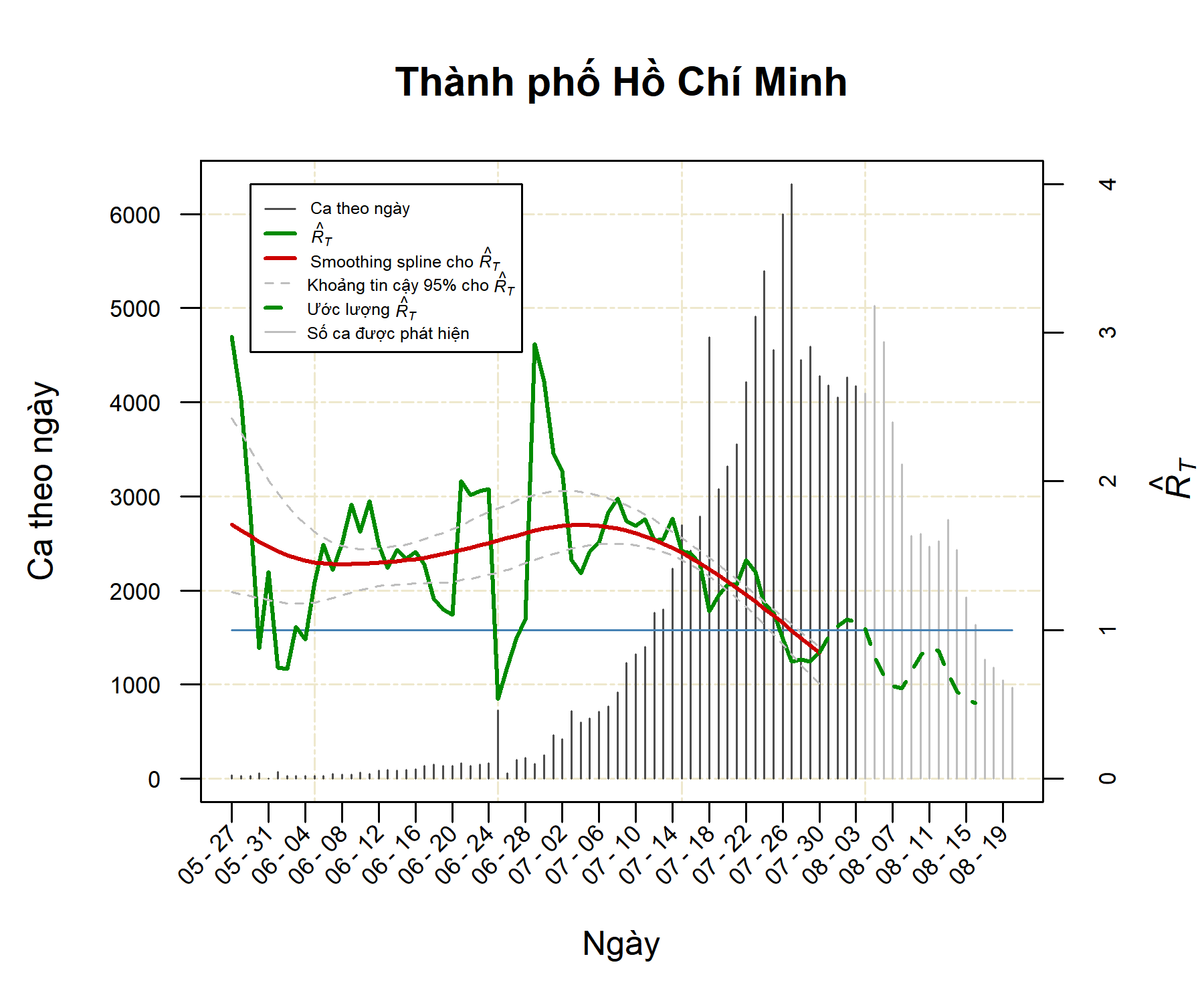
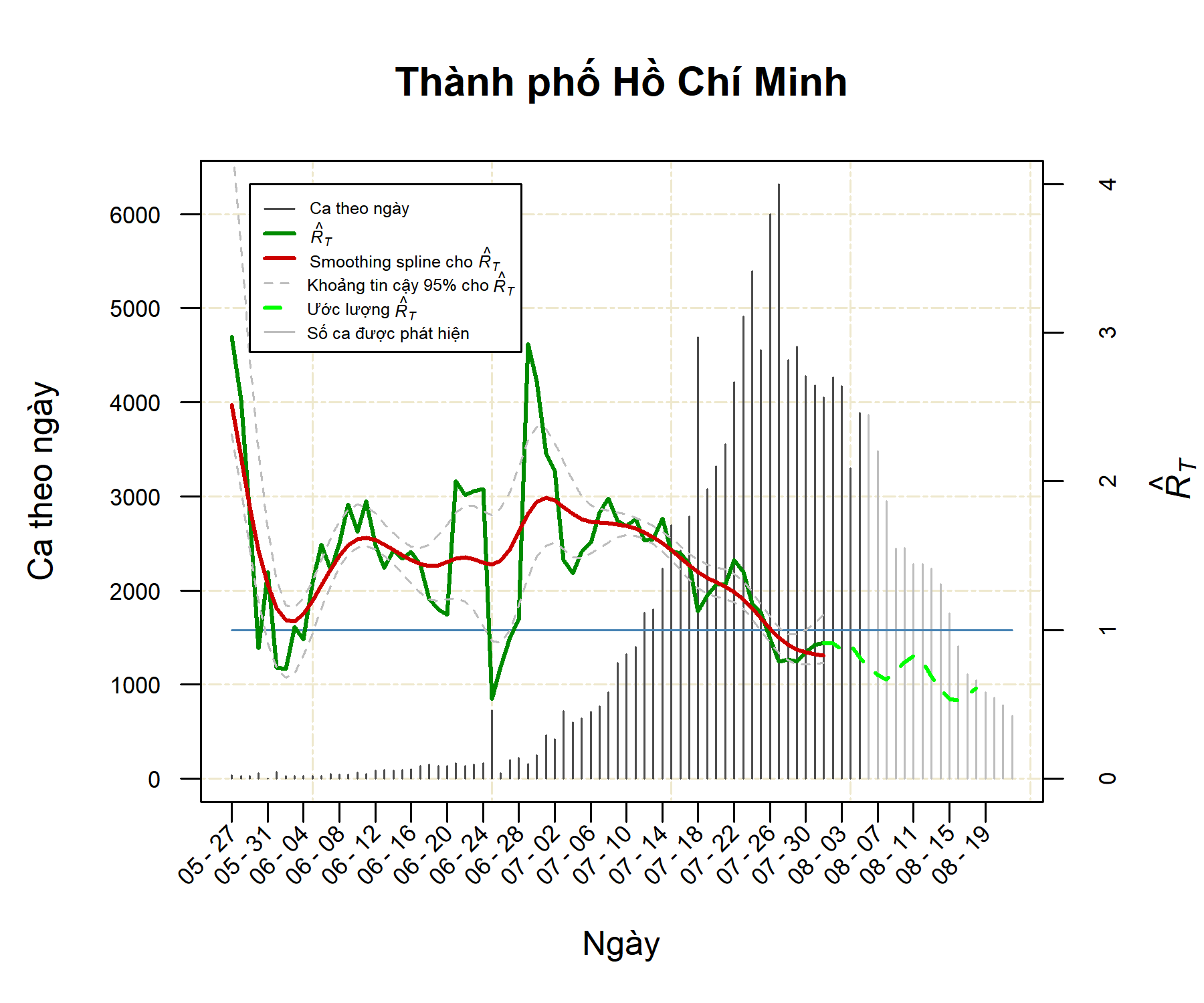
Figure 5. Wave prediction for HCMC.

2.5. Lockdown timing

There is research on how many days before the epidemic peak to impose a lockdown, but we have not found research on choosing the lockdown day according to the epidemic cycle ⁵. To illustrate, let us consider a simple example.

Example 4: One hundred newly infected people enter society at time 0. A person infected at time t only infects one other person at time t + 4. Consider the following lockdown strategies:

We lock down on days 1 – 3, then lift the lockdown on day 4. The 100 people above will all infect healthy people on day 4. The 3-day lockdown is useless.
We do not intervene on days 1 – 3, but lock down on exactly day 4, then lift the lockdown from day 5 onward. The epidemic ends.
We hesitate and start the lockdown late, on day 5. By then the infection process has completed one more cycle on day 4. If the reproduction number is 5, we now have 500 more cases.

In practice, the above example suggests that if we lock down exactly on the day with the largest number of transmissions, we minimize the large number of cases created and control the epidemic faster. For example, a day with a sudden spike in cases (a sign of an SS). If the cycle is 4 days and the SS detection delay is 10 days, the next important transmission cycle will occur 2 days later. Another way that does not depend on the detection delay is to predict the trough of the green curve of R_T. If we are still hesitant about whether to lock down, we can consider an immediate temporary 2-day lockdown (exactly when we predict the local trough of the green curve) upon detecting a sudden spike in cases, to interrupt one strong transmission cycle. Then we reopen to reassess the situation.

Next we present two observations from real data. First, observe the green curve trajectory in Figure 5 for HCMC. It reached a local peak on 22/07 then went down. We speculated that it would go down for about 4 days then rise again, per observation. However, Directive 16+ applied on 24/07 kept it going down. In the end, it only truly rose again on 30/07. Because it fell for 7 days straight, when it rose again the green curve could no longer cross above 1. As a result, we only observe a local increase in cases instead of a local epidemic peak (which occurs when the green curve crosses above 1 and then back below 1).

We chose to analyze the outbreak in Delhi, India, from March – May because of some similarities. Delhi's total population is about 31 million and the highest daily case count was 28,395 on 20/04. The Delta variant was the main strain in that outbreak. The authorities applied some strong measures such as micro-containment zones and a night curfew on 05/04, which started bringing the reproduction number down. The authorities then imposed a complete lockdown at midnight on 19/04. Although the number of immune individuals in Delhi may be large due to previous outbreaks, simulation shows it does not affect the total case count much (since total new cases are still small relative to the population). We observed some phenomena similar to and different from HCMC. The green curve fell for 9 straight days from 13/04 to 23/4. The complete lockdown on 19/4 contributed to this decline. However, we are not yet sure why it fell for 6 straight days from 13 – 19/04. It may be because Delhi has the 7-day cycle phenomenon with low case numbers on Mondays (e.g., 19/04, 26/04, and 03/05).

Figure 6. The Delta outbreak from March – May in Delhi - India.

3. Conclusion

Scientifically, in this article we presented a way to estimate the serial interval, estimate the cases added by the SSE, and the daily case ups and downs caused by the SSE.

In addition, we simulated the phenomenon of the 7-day cycle overpowering the 4-day cycle of the green estimated curve for R_T. We also simulated the 4-day periodic phenomenon through Example 1 and commented on it through analysis of the HCMC outbreak.

We also made observations on how social behavior affects the epidemic cycle in section 2.5. Practically, the article helps us better understand the epidemic's spread mechanism as well as the interaction between society and the virus.

We regard the epidemic peak as when the red curve crosses down through exactly 1 (meaning the average trend falls below 1). Local epidemic peaks occur when the green curve rises above 1 and then falls below 1.

The article still has certain limitations, such as we have not yet found a way to quantitatively forecast the green curve precisely (the green curve's wave differs from the case count wave). This quantitative forecast also requires relatively large daily case numbers to remove noise. We assume the case counts on 25/06 and 03/07 in HCMC resulted from an SS, but this is not easy to verify.

We hope the article helps you think more carefully about going into crowds before a lockdown, not be surprised when case numbers climb abnormally, and worry less when seeing local epidemic peaks. Policymakers can assess the situation more accurately and devise more effective lockdown options (such as issuing market passes before a lockdown).

Preparing an article always takes time, so sometimes we publish early summaries on Facebook.

Website updating R_T and other indicators operating since 21/09/2021 at onyx.vn/covid19/
Appendix: Weekly updates of the reproduction number and forecasts for Vietnam, some provinces, and cities

References

1. CSSE, J. COVID-19 Data Repository by the Center for Systems Science and Engineering (CSSE) at Johns Hopkins University. (2020). Available at: https://github.com/CSSEGISandData/COVID-19/tree/master/csse_covid_19_data/csse_covid_19_daily_reports.

2. Google. Google Mobility - Community mobility trend reports during the COVID-19 pandemic.

3. Google. Coronavirus (COVID-19). Available at: https://news.google.com/covid19/map?hl=vi&gl=VN&ceid=VN%3Avi.

4. Ricon-Becker, I. et al. A seven-day cycle in COVID-19 infection, hospitalization, and mortality rates: Do weekend social interactions kill susceptible people? ORCID. Tel Aviv 69978,

5. Oraby, T. et al. Modeling the effect of lockdown timing as a COVID-19 control measure in countries with differing social contacts. Sci. Reports 2021 111 11, 1–13 (2021).